Transformers for the lazy and curious
Why transformers are useful
Transformers were revolutionary because they introduced a way to process sequential data in parallel.
Before transformers, the state of the art tools were RNNs and LSTMs, both of which processed each input token in sequence which was inefficient during training and during inference. The efficiency that this architectural paradigm provided is what made modern LLMs possible.
The Transformer architecture
The transformer architecture introduced in the original paper consists of two big parts. The encoder and the decoder. We will be going through each part in greater detail.
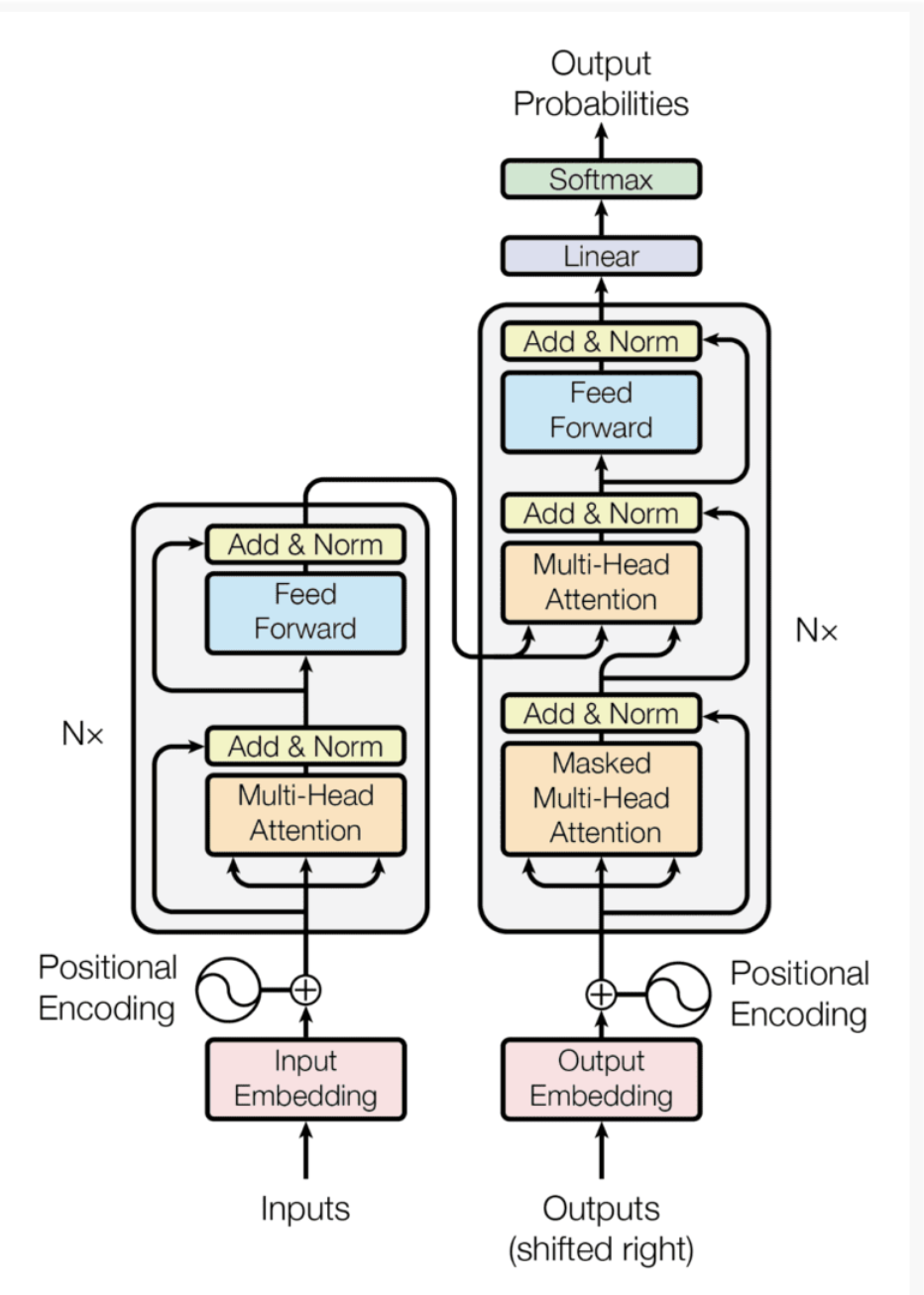
The full architecture in all its glory. The encoder is the block on the left and the decoder is the block on the right which is producing output
The Encoder
The encoder section consists of Nx blocks stacked on top of each other in sequence. In the orginal paper, Nx was 6. There is no real reason why this number was chosen. It was just what was tried.
The transformer with the encoder highlighted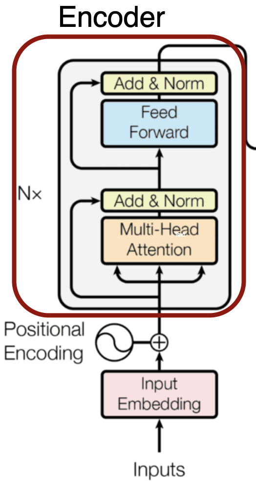
The entire input sequence is tokenized and passed into the encoder at once. When we refer to a context window with LLMs we are referring to the size limit of the input sequence that our model can support. The original paper used the variable $n$ to represent context length.
The first step is to convert the tokens into vectors. In the original paper, this was a vector of 512 dimensions, represented by the variable, $d_{model}$. This conversion is done by the input embedding. There are many different kinds of input embedding, however a good embedding will group semantically similar tokens together in the embedding space. We would expect a word like “human” to be closer to a word like “king” than it is to “dog”.
The next step is inject positional context. Recall that in transformers, the entire input sequence is passed in at once, not one at a time in sequence. The position of a token in the sequence has a large impact on the meaning of the sequence. We want to make sure we take this data into account.
In the original paper, the embedding vectors are augmented with positional context using sine and cosine functions of different frequencies.
Once positional context is added, the input goes to the multi-head attention layer. We will talk more about what attention is in a little while. At a high level, the attention block determines how each token in our sequence relates to the other tokens in the sequence. The add block that follows adds this information to the original embedding vectors, translating them in the embedding space to more accurately reflect their relative meaning in the input sequence. The normalization step that is done ensures that our vectors maintain a consistent mean and variance. This will ensure that they converge faster and speed up our training.
After the attention layer, the input is passed into a feed-forward layer. The feed-forward layer is a useful way to add non-linearity into our model. In the paper, they used a feed-forward layer with ReLU to add this non-linearity. The TLDR on why non-linearity is important is that non-linear activation functions allows your model to learn more complex patterns in your training data and thus produce better results.
This is a simple feed-forward network where each of the embedding vectors are passed through. Each of the vectors are passed through in parallel to speed things up but the feed-forward network is the same for all vectors. In the end you have an $n \times d_{model}$ sized matrix. There is an addition and normalization step right after which adds the values right before the feed forward layer and normalization for the same reason mentioned earlier.
At various points, we observe these skip connections or residual connections that connect the input to the output of a sub-block. This pattern, first introduced in the ResNet model is useful in preventing vanishing gradients. That’s why we have them here.
These same encoder steps are repeated $N_{x}$ times in sequence. At the end of this, we have a $n \times d_{model}$ matrix.
The Decoder
During inference, the input sequence is first processed by the encoder and then the decoder does generation. You can think of it as the encoder component is for “understanding” and the decoder is for responding.
Here’s a close up of the decoder.
The decoder sections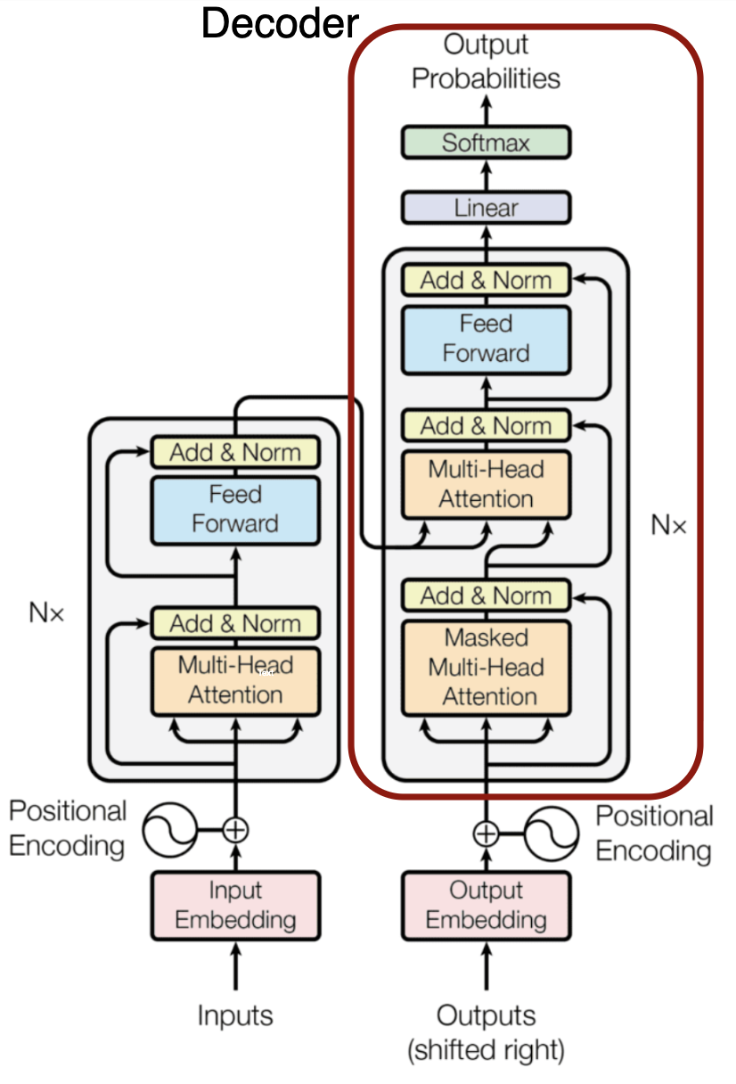
During inference, a single <start> token is passed in as input to the decoder. This input token is processed by the decoder and the next token is predicted. In the next time step the old input and the new output are concatenated and passed in as input to the decoder. This is the auto-regressive part of the transformer architecture. While during inference, each output token is generated one at a time, during training, we can actually run the decoder in parallel as we already know what the next token is and don’t need to wait to pass in the input at the next time step.
Let’s break down the core parts of the decoder. Like the encoder, our input first passes through embedding and positional encoding stages.
The input then passes through the first attention block. This block adds contextual meaning of a token within the sequence itself, same as in the encoder. So far, these two components are the same. The “masked” part of the attention block is mainly relevant for training. It means that while the entire training sequence is pushed into the decoder at once, only tokens that would have been generated are visible. The tokens that would have been generated in the future are masked or hidden. This prevents the decoder from peeking at the answer during training and overfitting.
The next attention block is referred to as the cross-attention block.
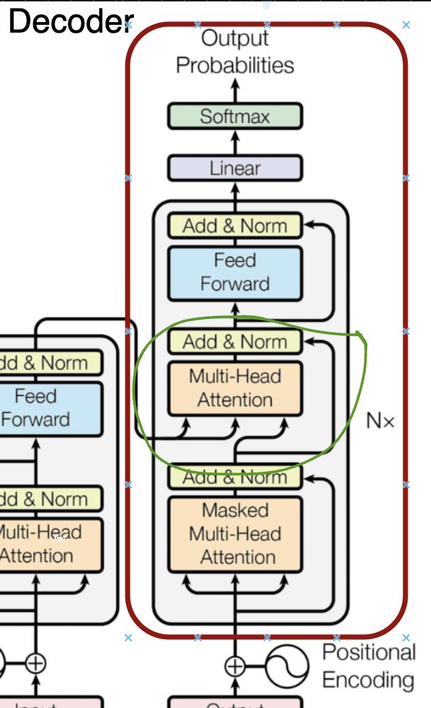
The cross attention block
The purpose of the cross-attention block is to allow the decoder to pull information from the original input sequence while it is generating the output sequence. It does this by having the decoder provide the query vectors while using the key and value vectors from the encoder. This type of attention block makes sense to use when we are attempting to go from one type of sequence into another type of sequence (ex. English to French translation).
After this step, standard addition and normalization are done followed by a feed-forward network to add non-linearity as before.
The output goes through $N_{x}$ stacks before going through a linear layer (basically a feed-forward layer) and then to a softmax layer to get next token probabilities.
How does Attention Work?
So far we have talked about how the major blocks of the transformer architecture fit together. However we only briefly discussed the attention mechanism.
The attention block receives an array of embedding vectors that represent the input sequence.
Let’s consider an example input sequence: “the king is old and sad”. This sequence will become an array of embedding vectors that we can represent as: $[\vec{E_{1}}, \vec{E_{2}}, \vec{E_{3}}, \vec{E_{4}}, \vec{E_{5}}, \vec{E_{6}}]$. We are assuming that every word corresponds to its own token.
For the moment, let’s consider just how the adjectives, “old” and “sad” modify the the embedding vector for “king”. This refers to a single head of attention. There can be many more dimensions, such as sentiment that can be used to update the meaning of the embedding vectors based on the surrounding vectors. These dimensions of meaning are not explicitly defined. Simply by adding multiple heads of attention, they arise. These multiple heads are what’s referred to as multi-headed attention.
To adjust the meaning of every token based its adjectives we need to first ask the question, for a given token, are there any adjectives that describe it? In the context of attention, this question is what is referred to as the query.
We have a query vector for every token in the sequence. We obtain this query vector by multiplying a matrix $W_{Q}$ by each embedding vector. At the end of this process we get an array of query vectors, one vector per token. The $W_{Q}$ matrix forms parameters of the model, which means its values are learned from data.
The query vector has a smaller dimension than the embedding vectors. In the original paper, the query vectors had a dimension of 64, compared to the 512 for the embedding space.
Along with the query vectors, we also have key vectors which exist for every token in the input sequence. Like the query vectors, these key vectors are obtained by multiplying a matrix of learned parameters, $W_{K}$.
We can think of the keys as matching the queries whenever they closely align with each other. In our example, which is focusing on adjectives acting on nouns, we would expect the key vectors for adjectives such as “old” and “sad” as mapping closely to the query vector for their noun, “king”.
To measure how well each key matches each query, we compute a dot product between each key query pair. In the end we end up with a table of values like the one shown below:
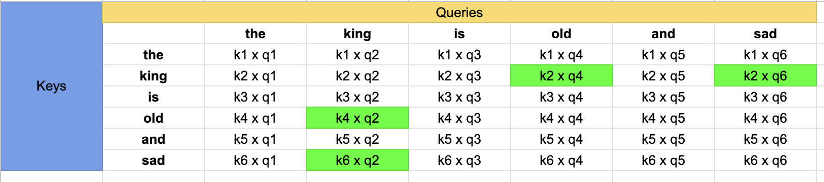
Key-Query dot product table
In this example, the keys that strongly inform (or to use the correct lingo - attend) a query result in a large positive value, and ones that don’t or are irrelevant produce small or negative values. In the end we have a table of values from $-\infty$ to $+\infty$ which represent a score correlating to how well a particular token relates to every other token.
We want to use these scores as a weighted sum along each column (query) for the keys of all the tokens. In order to do this, we want to convert the scores to be a number between 0 and 1 and have all the values in a column to add up to 1. To achieve this, we apply a softmax function along each of the columns.
An important thing to note is that when we are training our model, we use a technique called teacher forcing. We take an existing sequence and try to predict the next token for every possible sequence length. So we would have sequences like “the”, “the king”, “the king is” and so on. In this case, we do not want to consider tokens in the query-key table that occur after our sequence and so the model should not know about. We hide these tokens using a technique called masking, wherein we set these hidden query-key pairings to -inf so that they will always contribute a weight of 0. This is what the masked self-attention block in the decoder is doing.
Masked Key-Query dot product table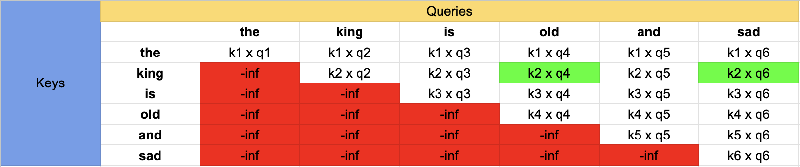
Once we have this query-key score table, we want a way to actually update the embedding vectors. This is where the value vector comes in. We do this by using another learned matrix called the value matrix, $W_{V}$. You multiply this value matrix by each embedding vector to get a vector $\vec{V_{i}}$ for each token. Looking back on query-key table, you multiply the resulting value vectors along each column and sum them to get the weighted value vector. This weighted value vector represents the delta that needs to be applied to the particular embedding vector to give it a more representative context. The delta is added to the embedding vector to get the updated embedding vector. We do this for all the embedding vectors to get the updated embedding vectors.
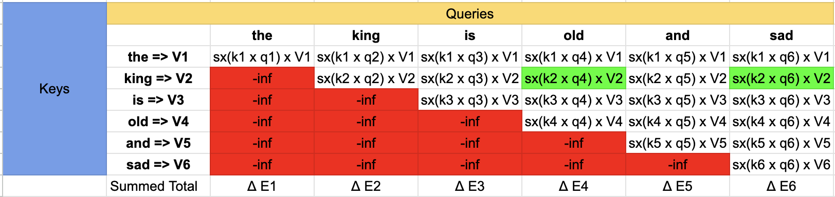
Adding value vectors to the embedding vectors. The sx is short for softmax
The original paper succinctly outlines the steps to compute the attention for each token as:
$$ \operatorname{Attention}(Q, K, V) = \operatorname{softmax}\left(\frac{QK^{\mathsf{T}}}{\sqrt{d_k}}\right)V $$
Note that there is a $\sqrt{d_k}$ that the query-key dot product gets divided by, making it a scaled-dot product. This is done simply to prevent the query-key scores from going to the extremes of the softmax function and resulting in non-informative values.